Vision Transformer：Transformer在计算机视觉的革命

引言

Transformer在NLP领域取得巨大成功后，研究者自然会思考：能否将Transformer应用到计算机视觉？

2020年，Google提出的Vision Transformer (ViT)给出了肯定的答案[1]，并掀起了CV领域的Transformer浪潮。2021年，微软的Swin Transformer更是将这一浪潮推向高潮，获得了ICCV 2021最佳论文奖[2]。

Vision Transformer (2020)

📄 论文信息

作者 Alexey Dosovitskiy, Lucas Beyer, Alexander Kolesnikov, Dirk Weissenborn, Xiaohua Zhai, Thomas Unterthiner, Mostafa Dehghani, Matthias Minderer, Georg Heigold, Sylvain Gelly, Jakob Uszkoreit, Neil Houlsby (Google Research)

发表 ICLR (2021)

论文 arXiv:2010.11929

arXiv 2010.11929

核心思想

An Image is Worth 16×16 Words：将图像看作序列！

Vision Transformer结构

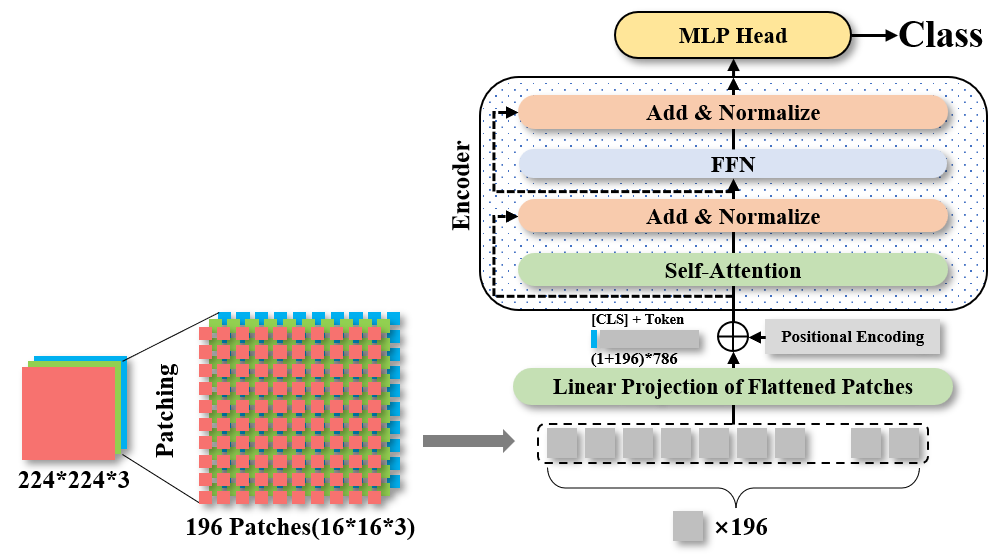
graph LR
    IMG["输入 224×224×3"] --> PATCH["Patch 分块<br/>16×16 → 196 patches"]
    PATCH --> CLS["+ [CLS] Token<br/>197 vectors"]
    CLS --> POS["+ 位置编码"]
    POS --> TRANS["Transformer ×12<br/>多头注意力 + MLP"]
    TRANS --> HEAD["分类头<br/>[CLS] → 线性层"]
    HEAD --> PRED["类别预测"]

架构设计

图像分块（Patch Embedding）

class PatchEmbedding(nn.Module):
    """将图像切分成patches并嵌入"""
    def __init__(self, img_size=224, patch_size=16, in_channels=3, embed_dim=768):
        super(PatchEmbedding, self).__init__()
        
        self.img_size = img_size
        self.patch_size = patch_size
        self.num_patches = (img_size // patch_size) ** 2
        
        # 使用卷积实现patch embedding
        self.proj = nn.Conv2d(in_channels, embed_dim, 
                             kernel_size=patch_size, stride=patch_size)
    
    def forward(self, x):
        # x: (batch, 3, 224, 224)
        x = self.proj(x)  # (batch, embed_dim, 14, 14)
        x = x.flatten(2)  # (batch, embed_dim, 196)
        x = x.transpose(1, 2)  # (batch, 196, embed_dim)
        return x

关键步骤：

224×224图像 → 切分成14×14=196个16×16的patches
每个patch展平成384维向量
线性投影到768维（embed_dim）

位置编码

class ViT(nn.Module):
    def __init__(self, img_size=224, patch_size=16, num_classes=1000, 
                 embed_dim=768, depth=12, num_heads=12):
        super(ViT, self).__init__()
        
        self.patch_embed = PatchEmbedding(img_size, patch_size, 3, embed_dim)
        num_patches = self.patch_embed.num_patches
        
        # Class token：可学习的分类token
        self.cls_token = nn.Parameter(torch.zeros(1, 1, embed_dim))
        
        # Position embedding：可学习的位置编码
        self.pos_embed = nn.Parameter(torch.zeros(1, num_patches + 1, embed_dim))
        
        # Transformer Encoder
        self.transformer = nn.TransformerEncoder(
            nn.TransformerEncoderLayer(embed_dim, num_heads, dim_feedforward=embed_dim*4),
            num_layers=depth
        )
        
        # Classification head
        self.norm = nn.LayerNorm(embed_dim)
        self.head = nn.Linear(embed_dim, num_classes)
    
    def forward(self, x):
        batch_size = x.shape[0]
        
        # Patch embedding
        x = self.patch_embed(x)  # (batch, 196, 768)
        
        # 添加class token
        cls_tokens = self.cls_token.expand(batch_size, -1, -1)  # (batch, 1, 768)
        x = torch.cat([cls_tokens, x], dim=1)  # (batch, 197, 768)
        
        # 添加位置编码
        x = x + self.pos_embed
        
        # Transformer
        x = self.transformer(x)
        
        # 分类
        x = self.norm(x)
        cls_token_final = x[:, 0]  # 只取class token
        x = self.head(cls_token_final)
        
        return x

核心组件

Class Token

思想：借鉴BERT的[CLS] token

在序列开头添加一个可学习的token
用于聚合整个序列的信息
最后用于分类

Position Embedding

ViT使用可学习的位置编码：

# 1D位置编码（每个patch一个）
self.pos_embed = nn.Parameter(torch.zeros(1, 197, 768))

与Transformer的区别：

Transformer：使用固定的sin/cos编码
ViT：使用可学习的编码

ViT的配置

| 模型 | 层数 | 隐藏维度 | MLP维度 | 头数 | 参数量 | |——|——|———|———|——|——–| | ViT-Base | 12 | 768 | 3072 | 12 | 86M | | ViT-Large | 24 | 1024 | 4096 | 16 | 307M | | ViT-Huge | 32 | 1280 | 5120 | 16 | 632M | [1]

核心发现

ViT论文的核心观点：

当拥有足够多的数据进行预训练时，ViT的表现会超过CNN。[1]

数据需求

| 数据集规模 | ViT表现 | ResNet表现 | |———–|———|———–| | ImageNet (1.2M) | 较差 | ✅ 好 | | ImageNet-21K (14M) | 相当 | ✅ 好 | | JFT-300M (300M) | ✅ 更好 | 好 | [1]

结论：ViT需要大规模预训练！

归纳偏置（Inductive Bias）

CNN的归纳偏置：

局部性（Locality）：相邻像素相关
平移不变性（Translation Equivariance）：卷积核共享

ViT的归纳偏置：

更少的归纳偏置
更依赖数据来学习
在大数据下有优势

模型复现

代码地址：GitHub - DeepLearning/model_classification/VisionTransformer

Swin Transformer (2021)

📄 论文信息

作者 Ze Liu, Yutong Lin, Yue Cao, Han Hu, Yixuan Wei, Zheng Zhang, Stephen Lin, Baining Guo (Microsoft Research Asia)

发表 ICCV (2021)

论文 arXiv:2103.14030

arXiv 2103.14030

荣誉：ICCV 2021 最佳论文 (Marr Prize)

核心问题

ViT的问题：

计算复杂度高：全局注意力复杂度O(n²)
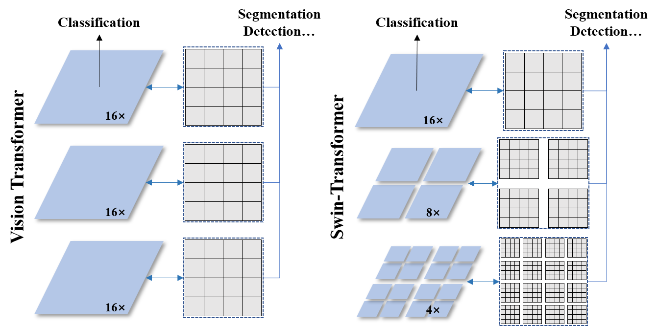
特征单一：只有16倍下采样，不适合密集预测
缺少层次化结构：不像CNN有多尺度特征

核心创新

Swin Transformer结构

窗口多头自注意力（W-MSA）

Swin Feature Maps

思想：将图像划分成不重叠的窗口，只在窗口内计算注意力。

def window_partition(x, window_size):
    """
    将特征图划分成窗口
    x: (B, H, W, C)
    window_size: 窗口大小M
    返回: (B*num_windows, M, M, C)
    """
    B, H, W, C = x.shape
    x = x.view(B, H // window_size, window_size, W // window_size, window_size, C)
    windows = x.permute(0, 1, 3, 2, 4, 5).contiguous()
    windows = windows.view(-1, window_size, window_size, C)
    return windows

def window_reverse(windows, window_size, H, W):
    """
    将窗口还原成特征图
    """
    B = int(windows.shape[0] / (H * W / window_size / window_size))
    x = windows.view(B, H // window_size, W // window_size, window_size, window_size, -1)
    x = x.permute(0, 1, 3, 2, 4, 5).contiguous().view(B, H, W, -1)
    return x

复杂度分析：

全局注意力（ViT）： \(\text{FLOPs} = 4hwC^2 + 2(hw)^2C\)

窗口注意力（Swin）： \(\text{FLOPs} = 4hwC^2 + 2hwM^2C\)

差距：(2(hw)^2C - 2hwM^2C)

当h=w=56, M=7时，节省约49倍！

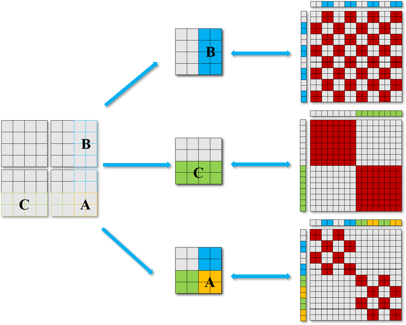
滑动窗口多头自注意力（SW-MSA）

SW-MSA

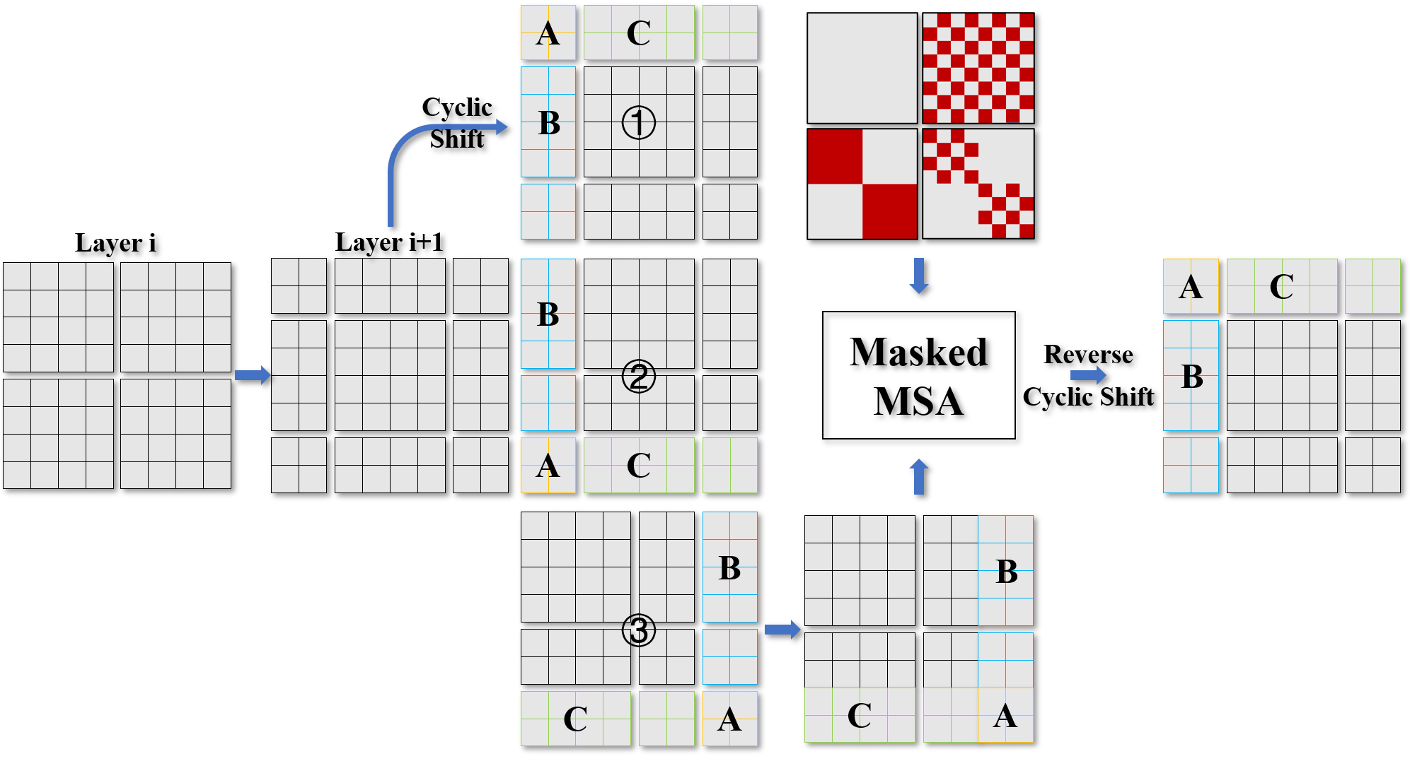
问题：W-MSA隔绝了窗口之间的信息交流。

解决：滑动窗口！

循环移位机制：

Cyclic Shift

class SwinTransformerBlock(nn.Module):
    def __init__(self, dim, num_heads, window_size=7, shift_size=0):
        super(SwinTransformerBlock, self).__init__()
        
        self.dim = dim
        self.num_heads = num_heads
        self.window_size = window_size
        self.shift_size = shift_size
        
        self.norm1 = nn.LayerNorm(dim)
        self.attn = WindowAttention(dim, window_size, num_heads)
        self.norm2 = nn.LayerNorm(dim)
        self.mlp = MLP(dim, dim * 4)
    
    def forward(self, x):
        H, W = self.H, self.W
        B, L, C = x.shape
        
        shortcut = x
        x = self.norm1(x)
        x = x.view(B, H, W, C)
        
        # 循环移位
        if self.shift_size > 0:
            shifted_x = torch.roll(x, shifts=(-self.shift_size, -self.shift_size), dims=(1, 2))
        else:
            shifted_x = x
        
        # 窗口划分
        x_windows = window_partition(shifted_x, self.window_size)
        x_windows = x_windows.view(-1, self.window_size * self.window_size, C)
        
        # W-MSA/SW-MSA
        attn_windows = self.attn(x_windows)
        
        # 窗口还原
        attn_windows = attn_windows.view(-1, self.window_size, self.window_size, C)
        shifted_x = window_reverse(attn_windows, self.window_size, H, W)
        
        # 反向循环移位
        if self.shift_size > 0:
            x = torch.roll(shifted_x, shifts=(self.shift_size, self.shift_size), dims=(1, 2))
        else:
            x = shifted_x
        
        x = x.view(B, H * W, C)
        
        # 残差连接
        x = shortcut + x
        x = x + self.mlp(self.norm2(x))
        
        return x

Patch Merging

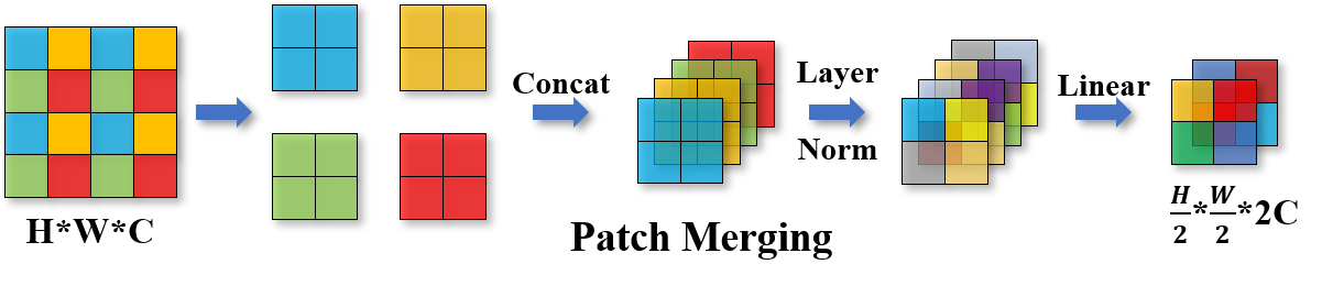
思想：构建层次化特征，类似CNN的下采样。

class PatchMerging(nn.Module):
    """下采样模块：2x2邻域合并"""
    def __init__(self, dim):
        super(PatchMerging, self).__init__()
        self.dim = dim
        self.reduction = nn.Linear(4 * dim, 2 * dim, bias=False)
        self.norm = nn.LayerNorm(4 * dim)
    
    def forward(self, x, H, W):
        """
        x: (B, H*W, C)
        """
        B, L, C = x.shape
        x = x.view(B, H, W, C)
        
        # 2x2邻域采样
        x0 = x[:, 0::2, 0::2, :]  # (B, H/2, W/2, C)
        x1 = x[:, 1::2, 0::2, :]
        x2 = x[:, 0::2, 1::2, :]
        x3 = x[:, 1::2, 1::2, :]
        
        x = torch.cat([x0, x1, x2, x3], dim=-1)  # (B, H/2, W/2, 4C)
        x = x.view(B, -1, 4 * C)
        
        x = self.norm(x)
        x = self.reduction(x)  # (B, H/2*W/2, 2C)
        
        return x

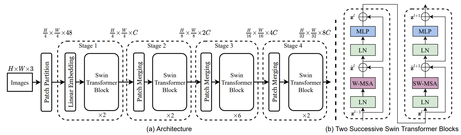
Swin Transformer完整架构

graph LR
    INPUT["224×224×3"] --> S1["Stage 1<br/>Patch Partition + Linear<br/>56×56×96 · ×2 Blocks"]
    S1 --> PM1["Patch Merging"]
    PM1 --> S2["Stage 2<br/>28×28×192 · ×2 Blocks"]
    S2 --> PM2["Patch Merging"]
    PM2 --> S3["Stage 3<br/>14×14×384 · ×6 Blocks"]
    S3 --> PM3["Patch Merging"]
    PM3 --> S4["Stage 4<br/>7×7×768 · ×2 Blocks"]

Swin的配置

| 模型 | C | 层数配置 | 参数量 | FLOPs | |——|—|———|——–|——-| | Swin-T | 96 | 2,2,6,2 | 29M | 4.5G | | Swin-S | 96 | 2,2,18,2 | 50M | 8.7G | | Swin-B | 128 | 2,2,18,2 | 88M | 15.4G | | Swin-L | 192 | 2,2,18,2 | 197M | 34.5G | [2]

相对位置偏置

Swin使用相对位置偏置（Relative Position Bias）：

\[\text{Attention}(Q, K, V) = \text{SoftMax}\left(\frac{QK^T}{\sqrt{d}} + B\right)V\]

其中B是可学习的相对位置偏置矩阵。

# 相对位置偏置
self.relative_position_bias_table = nn.Parameter(
    torch.zeros((2 * window_size - 1) * (2 * window_size - 1), num_heads)
)

性能对比

ImageNet分类

| 模型 | 参数量 | FLOPs | Top-1准确率 | |——|——–|——-|———–| | ResNet-50 | 25M | 4.1G | 79.8% | | ViT-B | 86M | 17.6G | 81.8% | | Swin-T | 29M | 4.5G | 81.3% | | Swin-B | 88M | 15.4G | 83.5% | [1],[2]

COCO目标检测

| Backbone | 参数量 | FLOPs | AP | |———-|——–|——-|—–| | ResNet-50 | 44M | 260G | 46.0 | | ViT-B | 115M | 360G | 48.7 | | Swin-T | 48M | 264G | 50.5 | [1],[2]

Swin在下游任务上表现更好！

模型复现

代码地址：GitHub - DeepLearning/model_classification/SwinTransformer

ViT vs Swin Transformer

维度	ViT	Swin Transformer
注意力范围	全局	局部（窗口）
计算复杂度	O(n²)	O(n)
特征层次	单一（16×）	多尺度（4×,8×,16×,32×）
数据需求	极大	较大
下游任务	分类优秀	检测/分割更好
归纳偏置	少	适中

Transformer vs CNN

CNN的优势

✅ 归纳偏置强：局部性、平移不变性 ✅ 数据效率高：小数据也能训练 ✅ 计算高效：参数共享

Transformer的优势

✅ 全局建模：长距离依赖 ✅ 扩展性好：数据越多越强 ✅ 灵活性高：统一架构

未来趋势

混合架构：结合CNN和Transformer的优势

ConvNeXt：现代化CNN
CoAtNet：卷积+注意力
CMT：卷积+多头注意力

实践经验

何时使用ViT/Swin？

✅ 适用场景：

大规模预训练
需要全局信息
下游任务多样

❌ 不适用：

数据量小
计算资源受限
需要实时推理

预训练策略

# 使用ImageNet-21K预训练
model = timm.create_model('swin_base_patch4_window7_224_in22k', pretrained=True)

# 在自己的数据上微调
model.head = nn.Linear(model.head.in_features, num_classes)

数据增强

Transformer需要更强的数据增强：

from timm.data import create_transform

transform = create_transform(
    input_size=224,
    is_training=True,
    auto_augment='rand-m9-mstd0.5-inc1',  # AutoAugment
    re_prob=0.25,  # Random Erasing
    mixup_alpha=0.8,  # Mixup
    cutmix_alpha=1.0  # CutMix
)

优化技巧

# 1. 使用AdamW优化器
optimizer = torch.optim.AdamW(model.parameters(), lr=1e-3, weight_decay=0.05)

# 2. Cosine学习率
scheduler = torch.optim.lr_scheduler.CosineAnnealingLR(optimizer, T_max=epochs)

# 3. Warmup
warmup_epochs = 20
for epoch in range(warmup_epochs):
    lr = base_lr * (epoch + 1) / warmup_epochs
    for param_group in optimizer.param_groups:
        param_group['lr'] = lr

# 4. Layer-wise LR Decay
for layer_id, (name, param) in enumerate(model.named_parameters()):
    lr_scale = 0.95 ** (num_layers - layer_id)
    param_group = {'params': param, 'lr': base_lr * lr_scale}

总结

Vision Transformer的贡献

证明了Transformer在CV的可行性
打破了CNN的垄断
启发了大量后续研究
推动了视觉-语言统一建模

Swin Transformer的贡献

窗口注意力机制：降低复杂度
层次化设计：适合密集预测
相对位置偏置：更好的位置建模
SOTA性能：多个任务刷新记录

关键启示

Transformer是通用架构：不只是NLP
归纳偏置的权衡：少vs多，数据vs先验
层次化很重要：多尺度特征不可或缺
局部+全局：窗口注意力的智慧

影响与展望

Transformer在CV的影响

📊 刷新了多个视觉任务的SOTA
🔧 催生了大量Transformer变体
🚀 推动了视觉基础模型的发展
🎓 统一了视觉和语言的架构

未来方向

效率优化：降低计算复杂度
小数据学习：减少数据依赖
多模态融合：视觉+语言+…
可解释性：理解Transformer学到了什么

参考文献

Dosovitskiy, A. et al. An Image is Worth 16x16 Words: Transformers for Image Recognition at Scale. ICLR, 2021. arXiv: 2010.11929
Liu, Z. et al. Swin Transformer: Hierarchical Vision Transformer using Shifted Windows. ICCV, 2021. arXiv: 2103.14030