MobileNet系列:移动端的深度学习革命
MobileNet系列:移动端的深度学习革命
引言
在经历了GoogLeNet多年多个版本的递进研究后,深度学习各模型之间的竞争大多集中在大规模计算和硬件算力上。2017年,Google团队转而将目光投向了深度学习在小规模计算集群的部署上。
MobileNet,正如其名——可以在移动设备上部署的深度学习网络。Google团队通过创新的网络设计,让算力较低的设备(如手机和小型电脑)也能完成深度学习任务。
系列概览
论文列表
- [2017] MobileNet V1:MobileNets: Efficient Convolutional Neural Networks for Mobile Vision Applications
- [2018] MobileNet V2:MobileNetV2: Inverted Residuals and Linear Bottlenecks
- [2019] MobileNet V3:Searching for MobileNetV3
MobileNet V1 (2017)
设计目标
- ✅ 减少参数量
- ✅ 降低计算量
- ✅ 保持合理的精度
- ✅ 适合移动端部署
核心创新:深度可分离卷积
MobileNet V1的核心是深度可分离卷积(Depthwise Separable Convolution) [1]。
标准卷积的问题
标准卷积的计算量:
\[\text{Params} = K \times K \times M \times N\] \[\text{FLOPs} = K \times K \times M \times N \times H \times W\]其中:
- (K\times K):卷积核大小
- (M):输入通道数
- (N):输出通道数(卷积核个数)
- (H \times W):特征图尺寸
深度可分离卷积
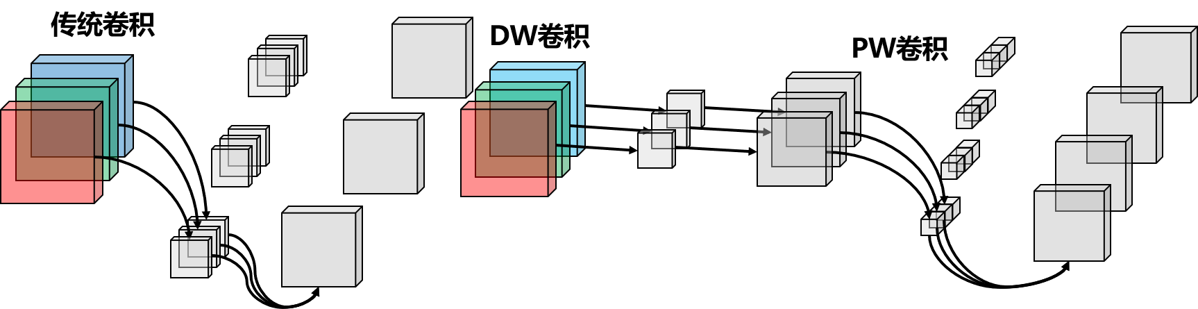
深度可分离卷积 = 深度卷积(DW) + 逐点卷积(PW)
1. 深度卷积(Depthwise Convolution, DW)
思想:每个输入通道使用独立的卷积核。
# DW卷积:每个通道独立处理
nn.Conv2d(in_channels=M, out_channels=M,
          kernel_size=3, groups=M)  # groups=M是关键
计算量: \(\text{FLOPs}_{DW} = K \times K \times M \times H \times W\)
2. 逐点卷积(Pointwise Convolution, PW)
思想:使用1×1卷积进行通道间信息融合。
# PW卷积:1×1卷积
nn.Conv2d(in_channels=M, out_channels=N, kernel_size=1)
计算量: \(\text{FLOPs}_{PW} = M \times N \times H \times W\)
计算量对比
总计算量: \(\text{FLOPs}_{DSC} = K^2 \cdot M \cdot H \cdot W + M \cdot N \cdot H \cdot W\)
压缩比: \(\frac{\text{FLOPs}_{DSC}}{\text{FLOPs}_{Standard}} = \frac{1}{N} + \frac{1}{K^2}\)
当(K=3)时,压缩比约为 1/9!
graph LR
    subgraph STD["标准卷积"]
        S_IN["M 通道"] --> S_C["K×K Conv<br/>M×N kernels"]
        S_C --> S_OUT["N 通道<br/>FLOPs: K²·M·N·H·W"]
    end
    subgraph DSC["深度可分离卷积"]
        D_IN["M 通道"] --> DW["Depthwise<br/>K×K · groups=M<br/>FLOPs: K²·M·H·W"]
        DW --> PW["Pointwise<br/>1×1 · M→N<br/>FLOPs: M·N·H·W"]
        PW --> D_OUT["N 通道<br/>≈ 1/9 FLOPs"]
    end
    style STD fill:#fce4ec,stroke:#c62828
    style DSC fill:#e8f5e9,stroke:#2e7d32
网络结构
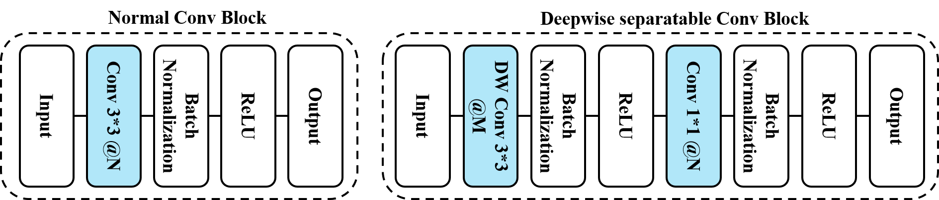
class DepthwiseSeparableConv(nn.Module):
    """深度可分离卷积模块"""
    def __init__(self, in_channels, out_channels, stride=1):
        super(DepthwiseSeparableConv, self).__init__()

        # Depthwise卷积
        self.depthwise = nn.Sequential(
            nn.Conv2d(in_channels, in_channels, kernel_size=3,
                     stride=stride, padding=1, groups=in_channels, bias=False),
            nn.BatchNorm2d(in_channels),
            nn.ReLU(inplace=True)
        )

        # Pointwise卷积
        self.pointwise = nn.Sequential(
            nn.Conv2d(in_channels, out_channels, kernel_size=1, bias=False),
            nn.BatchNorm2d(out_channels),
            nn.ReLU(inplace=True)
        )

    def forward(self, x):
        x = self.depthwise(x)
        x = self.pointwise(x)
        return x
模型复现
MobileNet V2 (2018)
核心创新
V2在V1的基础上提出了两个重要概念:
- Linear Bottleneck(线性瓶颈)
- Inverted Residual(逆残差结构)
问题:ReLU对低维信息的破坏
ReLU的非线性损失
ReLU激活函数会将负值全部置零: \(\text{ReLU}(x) = \max(0, x)\)
问题:当特征维度较低时,ReLU会丢失大量信息!

解决方案1:ReLU6
ReLU6定义: \(\text{ReLU6}(x) = \min(\max(0, x), 6)\)
# ReLU6实现
nn.ReLU6(inplace=True)
优势:
- 在6处截断,防止数值过大
- 减少精度损失
- 对低精度计算友好
解决方案2:逆残差结构
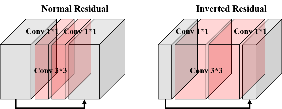
传统残差 vs 逆残差
| 维度 | 传统残差(ResNet) | 逆残差(MobileNet V2) |
|---|---|---|
| 路径 | 高维→低维→高维 | 低维→高维→低维 |
| 操作流程 | 降维→处理→升维 | 升维→处理→降维 |
| Shortcut | 高维 | 低维 |
| 核心思想 | 压缩表示 | 扩展表示 |
为什么要”逆”?
- DW卷积不改变通道数:需要先升维才能提取更丰富的特征
- 低维shortcut节省内存:低维的残差连接更高效
- 高维处理更有效:在高维空间进行特征提取效果更好
Inverted Residual Block
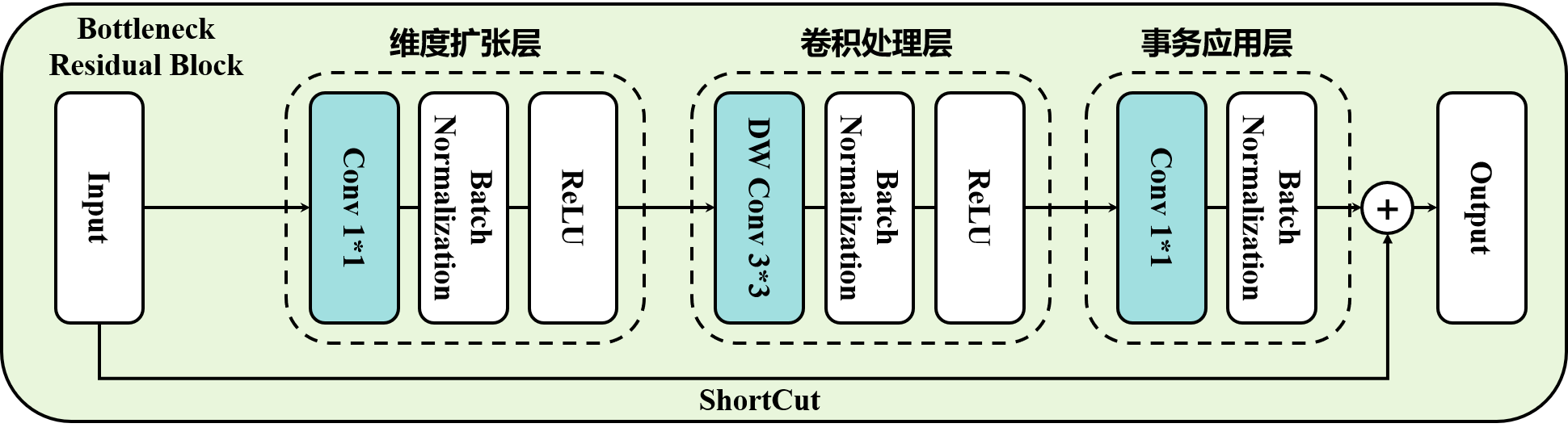
class InvertedResidual(nn.Module):
    """逆残差模块"""
    def __init__(self, in_channels, out_channels, stride, expand_ratio):
        super(InvertedResidual, self).__init__()

        hidden_dim = in_channels * expand_ratio
        self.use_residual = stride == 1 and in_channels == out_channels

        layers = []

        # 1. 升维(如果需要)
        if expand_ratio != 1:
            layers.append(nn.Sequential(
                nn.Conv2d(in_channels, hidden_dim, kernel_size=1, bias=False),
                nn.BatchNorm2d(hidden_dim),
                nn.ReLU6(inplace=True)
            ))

        # 2. Depthwise卷积
        layers.append(nn.Sequential(
            nn.Conv2d(hidden_dim, hidden_dim, kernel_size=3,
                     stride=stride, padding=1, groups=hidden_dim, bias=False),
            nn.BatchNorm2d(hidden_dim),
            nn.ReLU6(inplace=True)
        ))

        # 3. 降维(Linear Bottleneck)
        layers.append(nn.Sequential(
            nn.Conv2d(hidden_dim, out_channels, kernel_size=1, bias=False),
            nn.BatchNorm2d(out_channels),
            # 注意:这里没有ReLU!
        ))

        self.conv = nn.Sequential(*layers)

    def forward(self, x):
        if self.use_residual:
            return x + self.conv(x)
        else:
            return self.conv(x)
Linear Bottleneck
关键设计:最后的1×1卷积后不使用ReLU!
原因:
- 输出是低维的
- ReLU会破坏低维信息
- 使用线性激活保留更多信息
主要贡献
- 逆残差结构:更高效的特征提取
- Linear Bottleneck:保护低维信息
- ReLU6:更适合移动端的激活函数
- 更好的性能:参数量减少,精度提升
MobileNet V3 (2019)
核心创新
V3引入了三个主要改进 [3]:
- NAS(神经架构搜索)
- SE模块(Squeeze-and-Excitation)
- H-Swish激活函数
NAS - 神经架构搜索
暴力美学:使用优化算法自动搜索最优的网络结构。
搜索空间:
- 层数
- 卷积核大小
- 扩展比例
- 通道数
代价:需要极大的算力!
SE模块 - 通道注意力
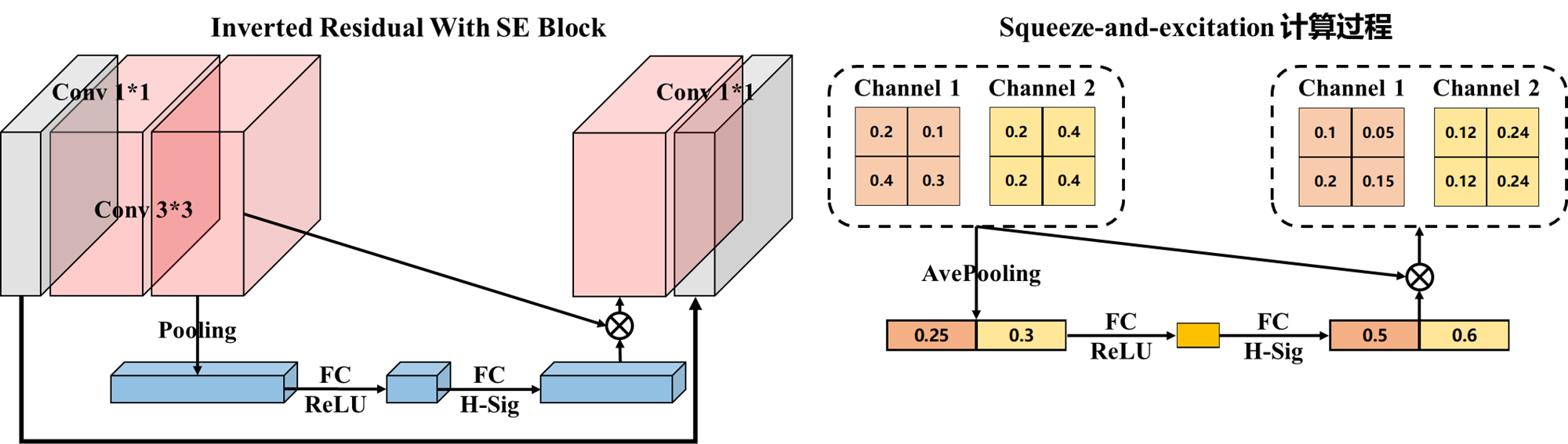
Squeeze-and-Excitation:学习通道之间的重要性。
class SEBlock(nn.Module):
    """SE注意力模块"""
    def __init__(self, channels, reduction=4):
        super(SEBlock, self).__init__()

        # Squeeze:全局平均池化
        self.avg_pool = nn.AdaptiveAvgPool2d(1)

        # Excitation:两层全连接
        self.fc = nn.Sequential(
            nn.Linear(channels, channels // reduction),
            nn.ReLU(inplace=True),
            nn.Linear(channels // reduction, channels),
            nn.Hardsigmoid(inplace=True)  # V3使用Hard-Sigmoid
        )

    def forward(self, x):
        b, c, _, _ = x.size()

        # Squeeze
        y = self.avg_pool(x).view(b, c)

        # Excitation
        y = self.fc(y).view(b, c, 1, 1)

        # Scale
        return x * y.expand_as(x)
H-Swish激活函数
Swish函数
标准Swish: \(\text{Swish}(x) = x \cdot \sigma(\beta x)\)
其中 (\sigma) 是Sigmoid函数。
问题:Sigmoid计算复杂,不适合移动端。
Hard-Swish
近似Swish: \(\text{H-Swish}(x) = x \cdot \frac{\text{ReLU6}(x + 3)}{6}\)
分段表达式: \(\text{H-Swish}(x) = \begin{cases} 0, & \text{if } x \leq -3 \\ x, & \text{if } x \geq 3 \\ \frac{x(x+3)}{6}, & \text{otherwise} \end{cases}\)
class HardSwish(nn.Module):
    def forward(self, x):
        return x * F.relu6(x + 3, inplace=True) / 6
优势:
- 计算简单(只需ReLU6)
- 硬件友好
- 效果接近Swish
MobileNet V3架构
V3提供两个版本:
- MobileNet V3-Large:高性能版本
- MobileNet V3-Small:高效版本
MobileNet系列对比
| 版本 | 核心技术 | 参数量(M) | 计算量(MFLOPs) | Top-1准确率 |
|---|---|---|---|---|
| V1 | DW+PW卷积 | 4.2 | 569 | 70.6% |
| V2 | 逆残差+Linear Bottleneck | 3.4 | 300 | 72.0% |
| V3-Large | NAS+SE+H-Swish | 5.4 | 219 | 75.2% |
| V3-Small | NAS+SE+H-Swish | 2.9 | 66 | 67.4% |
设计哲学的演进
V1:基础轻量化
- 目标:减少计算量
- 方法:深度可分离卷积
- 结果:计算量降到1/9
V2:特征表达优化
- 目标:保护信息同时降低计算量
- 方法:逆残差+Linear Bottleneck
- 结果:精度提升,计算量继续降低
V3:极致优化
- 目标:自动化设计+性能极致化
- 方法:NAS+SE+新激活函数
- 结果:精度和效率的最佳平衡
实践经验
选择合适的版本
# 场景1:高精度要求
model = mobilenet_v3_large(pretrained=True)

# 场景2:极致轻量
model = mobilenet_v3_small(pretrained=True)

# 场景3:平衡选择
model = mobilenet_v2(pretrained=True)
宽度乘数
MobileNet支持通过宽度乘数调整模型大小:
# 宽度乘数α:调整通道数
# α=1.0:标准模型
# α=0.75:减少25%通道
# α=0.5:减少50%通道

def adjust_channels(channels, width_mult=1.0):
    return int(channels * width_mult)
量化部署
# 动态量化
import torch.quantization

model_fp32 = mobilenet_v3_small(pretrained=True)
model_int8 = torch.quantization.quantize_dynamic(
    model_fp32,
    {nn.Linear, nn.Conv2d},
    dtype=torch.qint8
)

# 模型大小减少75%,速度提升2-4倍
迁移学习技巧
# 冻结特征提取层
model = mobilenet_v2(pretrained=True)

for param in model.features.parameters():
    param.requires_grad = False

# 只训练分类器
model.classifier = nn.Sequential(
    nn.Dropout(0.2),
    nn.Linear(model.last_channel, num_classes)
)
深度可分离卷积的应用
深度可分离卷积已成为轻量化网络的标准组件:
- ✅ MobileNet系列:开创者
- ✅ ShuffleNet:结合组卷积
- ✅ Xception:极致应用
- ✅ EfficientNet:NAS优化
优缺点分析
优点
- 参数量少:适合移动端部署
- 计算快:推理速度快
- 灵活性高:可调整宽度和分辨率
- 可扩展:易于修改和优化
缺点
- 精度略低:相比ResNet等大模型
- 实现复杂:特别是V3的SE模块和NAS
- 硬件依赖:需要硬件支持DW卷积
应用场景
MobileNet系列特别适合:
- 📱 移动应用:手机App中的AI功能
- 🤖 嵌入式系统:树莓派、IoT设备
- 🎥 实时视频处理:视频流分析
- 🚗 边缘计算:自动驾驶、智能监控
总结
技术演进
graph LR
    V1["V1 (2017)<br/>Depthwise Separable Conv<br/>DW + PW<br/>9× FLOPs 降低<br/>4.2M · 70.6%"] --> V2["V2 (2018)<br/>Inverted Residual<br/>Linear Bottleneck<br/>ReLU6<br/>3.4M · 72.0%"]
    V2 --> V3["V3 (2019)<br/>NAS + SE + H-Swish<br/>自动搜索架构<br/>5.4M · 75.2%"]
    style V1 fill:#e3f2fd,stroke:#1565c0
    style V2 fill:#e8f5e9,stroke:#2e7d32
    style V3 fill:#fff3e0,stroke:#e65100
核心思想
- 深度可分离卷积是关键:大幅降低计算量
- 逆残差很巧妙:更高效的特征提取
- 注意力机制有用:SE模块提升性能
- 自动化设计是趋势:NAS找到更优结构
影响
MobileNet系列:
- 📊 推动了移动端AI的发展
- 🔧 成为轻量化网络的设计范式
- 🚀 广泛应用于各类端侧场景
- 🎓 启发了众多后续研究
模型复现
我在PyTorch平台上复现了MobileNet系列:
- 平台:PyTorch
- 主要库:torchvision, torch, matplotlib, tqdm
- 数据集:Oxford Flower102花分类数据集
- 代码地址:GitHub - DeepLearning/model_classification/MobileNet
参考文献
- Howard, A. G., Zhu, M., Chen, B., Kalenichenko, D., Wang, W., Weyand, T., Andreetto, M., & Adam, H. MobileNets: Efficient Convolutional Neural Networks for Mobile Vision Applications. arXiv: 1704.04861, 2017.
- Sandler, M., Howard, A., Zhu, M., Zhmoginov, A., & Chen, L.-C. MobileNetV2: Inverted Residuals and Linear Bottlenecks. IEEE Conference on Computer Vision and Pattern Recognition (CVPR), 2018. arXiv: 1801.04381
- Howard, A., Sandler, M., Chu, G., Chen, L.-C., Chen, B., Tan, M., Wang, W., Zhu, Y., Pang, R., Vasudevan, V., Le, Q. V., & Adam, H. Searching for MobileNetV3. IEEE International Conference on Computer Vision (ICCV), 2019. arXiv: 1905.02244