Attention机制详解:深度学习的注意力革命
Attention机制详解:深度学习的注意力革命
引言
纵观深度学习发展历史,Google的贡献是无与伦比的。Attention机制最早出现在视觉领域[3],之后应用在自然语言处理领域,并成为现代深度学习最重要的组件之一。
Attention机制的产生背景
RNN的局限性
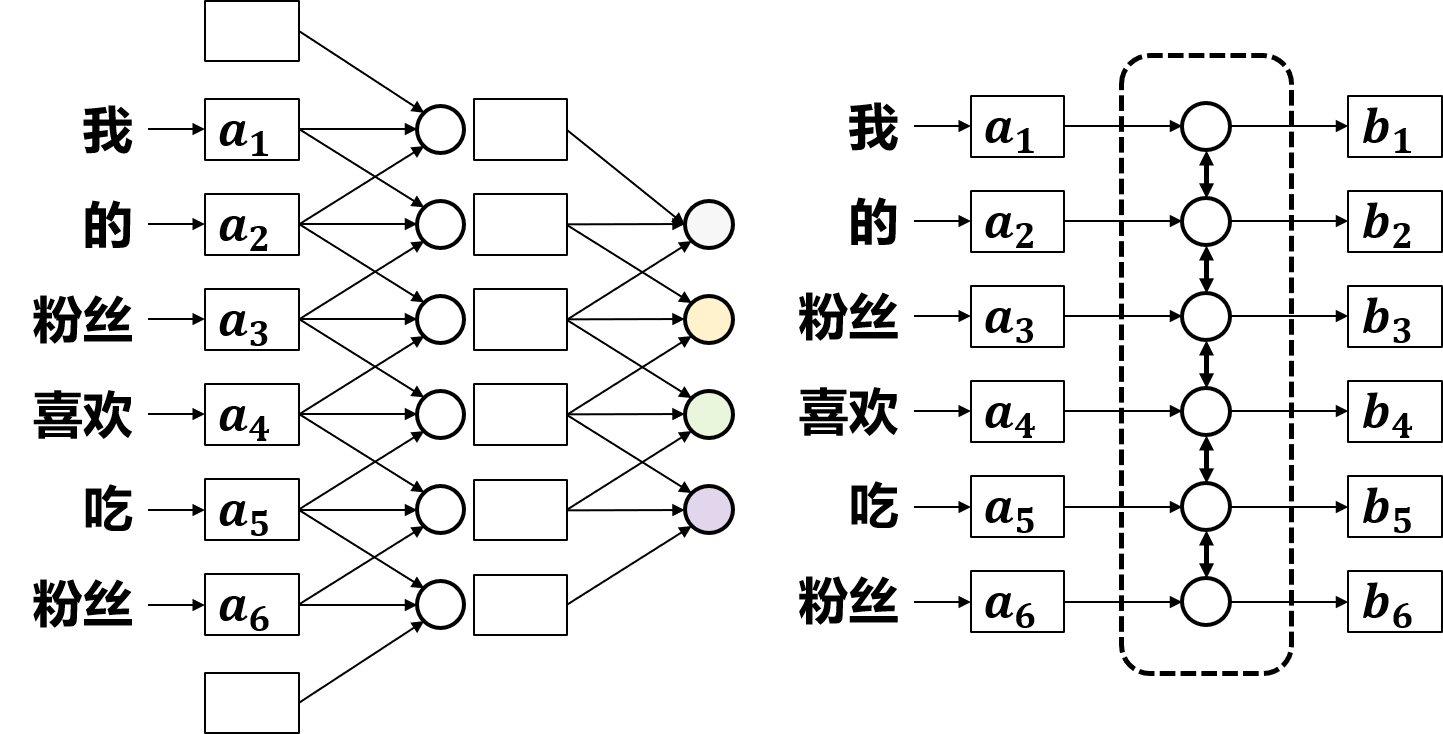
在NLP任务中,需要处理序列数据(Sequence):
RNN的问题
- 长期依赖问题:难以捕捉远距离的依赖关系
- 串行计算:无法并行,训练慢
- 信息瓶颈:固定长度的隐状态难以编码所有信息
- 等权重处理:所有输入被平等对待
关键问题:在序列中,不同位置的元素对当前预测的重要性是不同的!
Encoder-Decoder框架
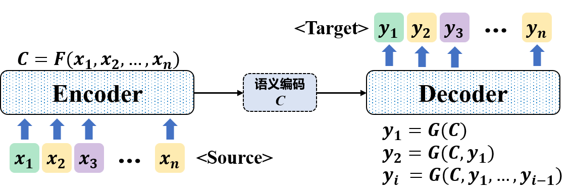
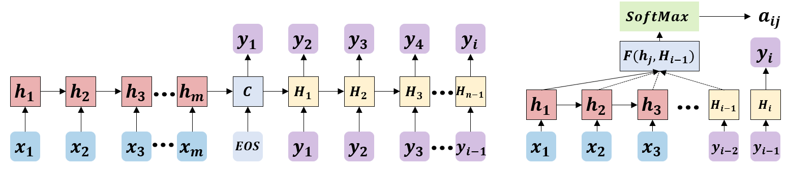
标准Encoder-Decoder(2014年提出)[1]:
\[\text{Encoder}: \mathbf{h}_t = f(\mathbf{x}_t, \mathbf{h}_{t-1})\] \[\text{Context}: \mathbf{c} = q(\mathbf{h}_1, ..., \mathbf{h}_T)\] \[\text{Decoder}: \mathbf{y}_t = g(\mathbf{c}, \mathbf{y}_1, ..., \mathbf{y}_{t-1})\]问题:所有 (\mathbf{y}_i) 都依赖于同一个固定的 (\mathbf{c}),权重相同!
Attention机制的核心思想
动态语义编码
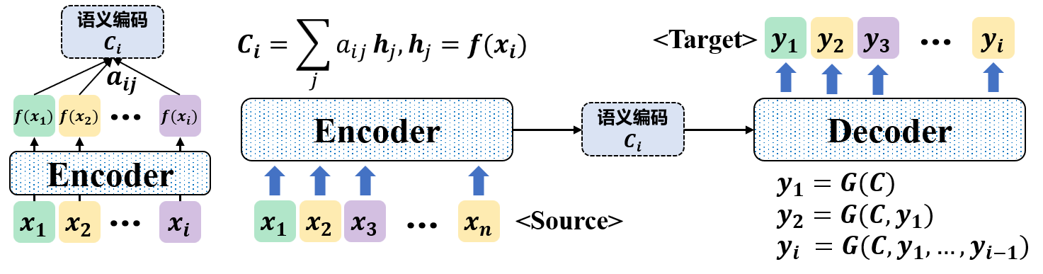
Attention的关键创新[1]:让每个输出关注不同的输入部分。
\[\mathbf{c}_i = \sum_{j=1}^{T_x} \alpha_{ij} \mathbf{h}_j\]其中 (\alpha_{ij}) 是注意力权重,表示生成 (\mathbf{y}_i) 时对 (\mathbf{h}_j) 的关注程度。
注意力权重的计算
第1步:计算相似度分数
\[e_{ij} = a(\mathbf{s}_{i-1}, \mathbf{h}_j)\]常用相似度函数:
- 点积:(a(\mathbf{s}, \mathbf{h}) = \mathbf{s}^T \mathbf{h})
- 缩放点积[2]:(a(\mathbf{s}, \mathbf{h}) = \frac{\mathbf{s}^T \mathbf{h}}{\sqrt{d}})
- 加性[1]:(a(\mathbf{s}, \mathbf{h}) = \mathbf{v}^T \tanh(\mathbf{W}_1\mathbf{s} + \mathbf{W}_2\mathbf{h}))
- 双线性:(a(\mathbf{s}, \mathbf{h}) = \mathbf{s}^T \mathbf{W} \mathbf{h})
第2步:归一化(Softmax)
\[\alpha_{ij} = \frac{\exp(e_{ij})}{\sum_{k=1}^{T_x} \exp(e_{ik})}\]第3步:加权求和
\[\mathbf{c}_i = \sum_{j=1}^{T_x} \alpha_{ij} \mathbf{h}_j\]Attention的本质
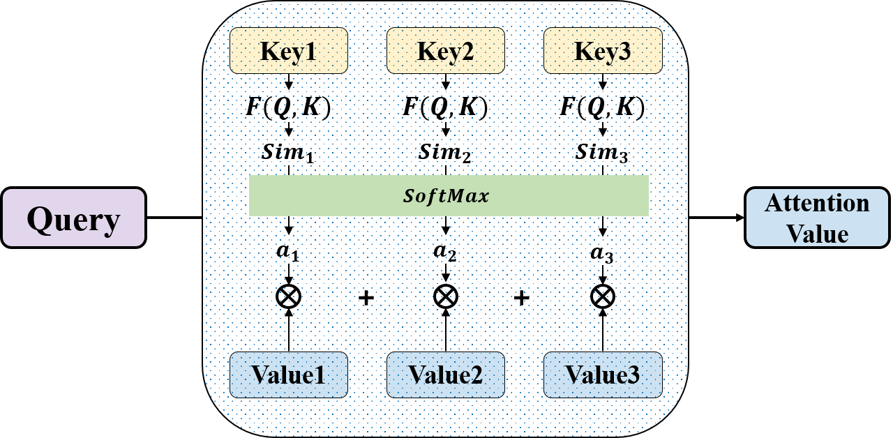
软寻址(Soft Addressing):
将Source看作存储器:
- Key:地址
- Value:内容
对于Query:
- 计算Query与每个Key的相似度
- 归一化得到注意力权重
- 对Value加权求和[2]
Attention的数学表达
通用公式
\[\text{Attention}(Q, K, V) = \sum_{i} \text{Similarity}(Q, K_i) \cdot V_i\]PyTorch实现
import torch
import torch.nn as nn
import torch.nn.functional as F

class BasicAttention(nn.Module):
    """基础的Attention机制"""
    def __init__(self, hidden_dim):
        super(BasicAttention, self).__init__()
        self.hidden_dim = hidden_dim

        # 注意力权重计算
        self.W_q = nn.Linear(hidden_dim, hidden_dim)
        self.W_k = nn.Linear(hidden_dim, hidden_dim)
        self.W_v = nn.Linear(hidden_dim, hidden_dim)

    def forward(self, query, key, value, mask=None):
        """
        query: (batch, query_len, hidden_dim)
        key: (batch, key_len, hidden_dim)
        value: (batch, value_len, hidden_dim)
        """
        # 1. 线性变换
        Q = self.W_q(query)  # (batch, query_len, hidden_dim)
        K = self.W_k(key)    # (batch, key_len, hidden_dim)
        V = self.W_v(value)  # (batch, value_len, hidden_dim)

        # 2. 计算注意力分数(缩放点积)
        scores = torch.matmul(Q, K.transpose(-2, -1))  # (batch, query_len, key_len)
        scores = scores / torch.sqrt(torch.tensor(self.hidden_dim, dtype=torch.float32))

        # 3. 应用mask(可选)
        if mask is not None:
            scores = scores.masked_fill(mask == 0, -1e9)

        # 4. Softmax归一化
        attention_weights = F.softmax(scores, dim=-1)  # (batch, query_len, key_len)

        # 5. 加权求和
        context = torch.matmul(attention_weights, V)  # (batch, query_len, hidden_dim)

        return context, attention_weights
Attention的变体
Self-Attention(自注意力)
特点[2]:Query、Key、Value来自同一个序列。
class SelfAttention(nn.Module):
    def __init__(self, hidden_dim):
        super(SelfAttention, self).__init__()
        self.attention = BasicAttention(hidden_dim)

    def forward(self, x, mask=None):
        # x: (batch, seq_len, hidden_dim)
        # Self-Attention: Q=K=V=x
        context, attention_weights = self.attention(x, x, x, mask)
        return context, attention_weights
应用:Transformer、BERT、GPT等。
Multi-Head Attention(多头注意力)
思想[2]:使用多组不同的Q、K、V矩阵,捕获不同的关系。
class MultiHeadAttention(nn.Module):
    """多头注意力机制"""
    def __init__(self, hidden_dim, num_heads):
        super(MultiHeadAttention, self).__init__()
        assert hidden_dim % num_heads == 0

        self.hidden_dim = hidden_dim
        self.num_heads = num_heads
        self.head_dim = hidden_dim // num_heads

        self.W_q = nn.Linear(hidden_dim, hidden_dim)
        self.W_k = nn.Linear(hidden_dim, hidden_dim)
        self.W_v = nn.Linear(hidden_dim, hidden_dim)
        self.W_o = nn.Linear(hidden_dim, hidden_dim)

    def split_heads(self, x):
        """分割成多个头"""
        batch_size, seq_len, hidden_dim = x.size()
        x = x.view(batch_size, seq_len, self.num_heads, self.head_dim)
        return x.transpose(1, 2)  # (batch, num_heads, seq_len, head_dim)

    def forward(self, query, key, value, mask=None):
        batch_size = query.size(0)

        # 1. 线性变换
        Q = self.W_q(query)
        K = self.W_k(key)
        V = self.W_v(value)

        # 2. 分割成多头
        Q = self.split_heads(Q)  # (batch, num_heads, query_len, head_dim)
        K = self.split_heads(K)
        V = self.split_heads(V)

        # 3. 缩放点积注意力
        scores = torch.matmul(Q, K.transpose(-2, -1))  # (batch, num_heads, query_len, key_len)
        scores = scores / torch.sqrt(torch.tensor(self.head_dim, dtype=torch.float32))

        if mask is not None:
            scores = scores.masked_fill(mask == 0, -1e9)

        attention_weights = F.softmax(scores, dim=-1)
        context = torch.matmul(attention_weights, V)  # (batch, num_heads, query_len, head_dim)

        # 4. 合并多头
        context = context.transpose(1, 2).contiguous()  # (batch, query_len, num_heads, head_dim)
        context = context.view(batch_size, -1, self.hidden_dim)  # (batch, query_len, hidden_dim)

        # 5. 输出投影
        output = self.W_o(context)

        return output, attention_weights
Cross-Attention(交叉注意力)
特点:Query来自一个序列,Key和Value来自另一个序列。
应用:机器翻译、图像字幕生成等。
Attention在NLP中的应用
机器翻译
在翻译”The cat sat on the mat”到”猫坐在垫子上”时:
- 翻译”猫”时,主要关注”cat”
- 翻译”坐”时,主要关注”sat”
- 翻译”垫子”时,主要关注”mat”
文本摘要
Attention帮助模型:
- 识别文章的关键句子
- 过滤冗余信息
- 生成简洁的摘要
问答系统
Attention帮助模型:
- 在文档中定位答案
- 理解问题与段落的关联
- 抽取或生成答案
Attention vs CNN vs RNN
| 特性 | CNN | RNN | Attention |
|---|---|---|---|
| 感受野 | 局部(可叠加为全局) | 全局(递归) | 全局(直接) |
| 并行性 | 高 | 低 | 高 |
| 长依赖 | 中等 | 差 | 好 |
| 计算复杂度 | O(n) | O(n) | O(n²) |
| 位置信息 | 隐式 | 隐式 | 需要显式编码 |
Attention的优势
解决长依赖问题
RNN的问题:信息经过多步传递会衰减。
Attention的解决:直接建立任意两个位置的连接。
提高并行性
RNN的问题:必须顺序计算。
Attention的解决:所有位置可以并行计算。
可解释性
可视化注意力权重:
import matplotlib.pyplot as plt
import seaborn as sns

def visualize_attention(attention_weights, source_tokens, target_tokens):
    """可视化注意力权重"""
    plt.figure(figsize=(10, 8))
    sns.heatmap(attention_weights,
                xticklabels=source_tokens,
                yticklabels=target_tokens,
                cmap='viridis',
                annot=True,
                fmt='.2f')
    plt.xlabel('Source')
    plt.ylabel('Target')
    plt.title('Attention Weights')
    plt.show()
性能提升
在各类NLP任务上,Attention都带来了显著的性能提升。
Attention的缺点
计算复杂度高
对于长度为n的序列:
- 空间复杂度:O(n²)
- 时间复杂度:O(n²·d)
缺少位置信息
Attention本身不考虑顺序,需要额外的位置编码。
训练数据需求
需要更多数据才能充分训练。
位置编码(Position Encoding)
为什么需要?
Attention是位置无关的,需要显式告诉模型位置信息。
绝对位置编码
Sinusoidal Position Encoding(Transformer使用):
\[PE(pos, 2i) = \sin\left(\frac{pos}{10000^{2i/d}}\right)\] \[PE(pos, 2i+1) = \cos\left(\frac{pos}{10000^{2i/d}}\right)\]class PositionalEncoding(nn.Module):
def __init__(self, d_model, max_len=5000):
super(PositionalEncoding, self).__init__()
# 创建位置编码矩阵
pe = torch.zeros(max_len, d_model)
position = torch.arange(0, max_len, dtype=torch.float).unsqueeze(1)
div_term = torch.exp(torch.arange(0, d_model, 2).float() *
(-math.log(10000.0) / d_model))
pe[:, 0::2] = torch.sin(position * div_term)
pe[:, 1::2] = torch.cos(position * div_term)
pe = pe.unsqueeze(0) # (1, max_len, d_model)
self.register_buffer('pe', pe)
def forward(self, x):
# x: (batch, seq_len, d_model)
x = x + self.pe[:, :x.size(1), :]
return x
可学习位置编码
class LearnedPositionalEncoding(nn.Module):
    def __init__(self, d_model, max_len=5000):
        super(LearnedPositionalEncoding, self).__init__()
        self.pos_embedding = nn.Embedding(max_len, d_model)

    def forward(self, x):
        # x: (batch, seq_len, d_model)
        batch_size, seq_len, _ = x.size()
        positions = torch.arange(seq_len, device=x.device).unsqueeze(0).repeat(batch_size, 1)
        x = x + self.pos_embedding(positions)
        return x
Attention的演进
graph LR
    A["2014: 基础 Attention"] --> B["2015: 各类变体"]
    B --> C["2017: Self-Attention / Transformer"]
    C --> D["2018: BERT"]
    D --> E["2019: GPT-2"]
    E --> F["2020: Vision Transformer"]
    F --> G["2021: Swin Transformer"]
总结
Attention的核心思想
- 选择性关注:不同输入有不同的重要性
- 动态权重:根据Query动态计算权重
- 软寻址:可微分的信息检索机制
关键组件
- Query(查询):我要什么?
- Key(键):我是什么?
- Value(值):我有什么?
计算流程
Query + Key → Similarity → Softmax → Weights
Weights + Value → Weighted Sum → Output
graph LR
    Q["Query<br/>我需要什么?"] --> SIM["点积相似度"]
    K["Key<br/>我是什么?"] --> SIM
    SIM --> SM["Softmax<br/>归一化"]
    SM --> W["注意力权重 αᵢⱼ"]
    V["Value<br/>我有什么?"] --> SUM["加权求和"]
    W --> SUM
    SUM --> OUT["输出 Context cᵢ"]
Attention的影响
Attention机制:
- 📊 成为现代NLP的核心组件
- 🔧 催生了Transformer革命
- 🚀 推动了大语言模型的发展
- 🎓 启发了众多后续研究
Attention改变了深度学习的范式!
实践建议
何时使用Attention?
✅ 适用场景:
- 序列到序列任务
- 长距离依赖
- 需要可解释性
- 变长输入
❌ 不适用:
- 极长序列(考虑稀疏Attention)
- 计算资源受限
- 位置信息极其重要
Attention的调优
# 1. 调整注意力头数
num_heads = 8  # 常用值:4, 8, 12, 16

# 2. 使用Dropout防止过拟合
attention = nn.Dropout(p=0.1)(attention)

# 3. 添加Layer Normalization
output = nn.LayerNorm(hidden_dim)(output)

# 4. 使用warmup学习率策略
scheduler = get_linear_schedule_with_warmup(optimizer, num_warmup_steps, num_training_steps)
参考文献
- Bahdanau, D., Cho, K., and Bengio, Y. Neural Machine Translation by Jointly Learning to Align and Translate. ICLR, 2015. arXiv: 1409.0473
- Vaswani, A., Shazeer, N., Parmar, N., Uszkoreit, J., Jones, L., Gomez, A. N., Kaiser, L., and Polosukhin, I. Attention Is All You Need. NeurIPS, 2017. arXiv: 1706.03762
- Mnih, V., Heess, N., Graves, A., and Kavukcuoglu, K. Recurrent Models of Visual Attention. NeurIPS, 2014. arXiv: 1406.6247